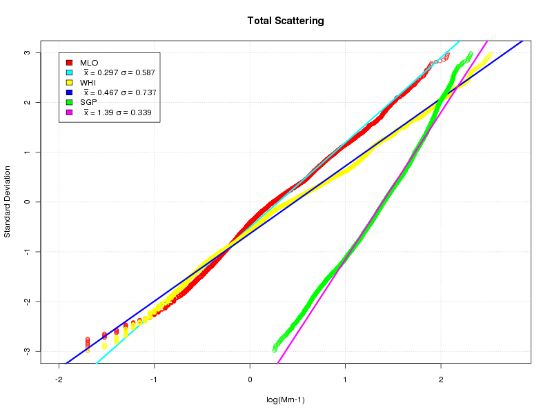
cdf_plot
cdf_plot generates a cumulative distribution plot for a single variable, with a y-axis scale that represents the inverse of the standard normal cumulative distribution for the corresponding value of the cumulative distribution function (CDF). It also plots a line with the same mean and standard deviation as the input data, to allow quick evaluation of the extent to which the data are normally distributed. It can accept one or multiple stations.
The transformation between the y-axis values and the cumulative distribution values is:
| y-value | cumulative fraction |
|---|---|
| 3 | 0.998650102 |
| 2 | 0.977249868 |
| 1 | 0.841344746 |
| 0 | 0.500000000 |
| -1 | 0.158655254 |
| -2 | 0.022750132 |
| -3 | 0.001349898 |
With the y-axis scale spanning the interval [-3,3], the plot displays over 99.7% of the input data.
Copy and modify the examples in /aer/prg/r/examples/cdf-stddev.r and /aer/prg/r/examples/multi-station-cdf-stddev.r if more customization is needed.
Command Line Usage
cdf_plot [--output=cdf.png] [--source=avgH] [--cut=0|1|disable]
         [--xtitle=""] [--maintitle=""] [--log] [--include=3]
         [--size=1024x768]
         station[,station2...] start end variable
Arguments
start and end
The time specifiers for the data to be retrieved. Start is inclusive while end is exclusive, so all data contained within the half open interval [start,end) will be used. Any convertible time format is accepted.
station[,station2...]
The station identifier code(s). For example 'brw'. Case insensitive. Multiple stations can be selected by separating them with “:”, “;” or “,”.
variable
The variable to plot. This should be specified without the cut size specifier if working with data that is split but cut size. For example, specifying 1um green scattering would be done like “–source=avgH –cut=1 … BsG_S11”.
--output=cdf.png
Set the output file name, defaulting to “cdf.png”.
--source=avgH
Set the source archive, defaulting to avgH.
--cut=0|1|disable
Set the cut size selection. Either 0 (PM10), 1 (PM1) or “disable” to use non-cut size split. Note that this must match what is available in the selected archive, so disable for scattering is not valid in hourly averages. Defaults to 0 for parameters that are cut size split and disable for those that aren't.
--xtitle=""
Set the X axis title.
--maintitle=""
Set the main plot title.
--log
Enable logarithmic (base 10) scaling on the X axis.
--include=3
Number of standard deviations out to include, defaulting to three. This defines the range of the Y-axis.
--size=1024x768
Set the output plot size.


